CS180: Project #2

Introduction

In this project, I explored various image processing techniques, including finite difference operators, derivative of Gaussian (DoG) filters, image sharpening, hybrid images, and multiresolution blending using Gaussian and Laplacian stacks. These techniques were applied to several images, such as the Cameraman, Apple, Orange, and some custom images, to analyze their effects on edge detection, frequency domain manipulation, and image blending. The following sections provide a detailed report of the methods and results.

Part 1: Fun with Filters

1.1 Finite Difference Operator

In this part, I used finite difference operators to approximate the gradients in the x and y directions of the image, detecting edges based on changes in intensity.

The partial derivatives were computed using theseg formulas: \[ \frac{\partial I}{\partial x} = I * D_x \\ \frac{\partial I}{\partial y} = I * D_y \\ \nabla I = \sqrt{\left( \frac{\partial I}{\partial x} \right)^2 + \left( \frac{\partial I}{\partial y} \right)^2} \] Here, \( D_x = [1, -1] \) and \( D_y = [1, -1]^T \), and convolution \( * \) is applied between the image and the derivative operators.

To highlight the edges, a threshold was applied to the gradient magnitude image which filtered out noise and helped us to focus on prominent edges. The thresholding allowed for clearer depiction of edges, although fine-tuning was necessary to achieve the right balance.

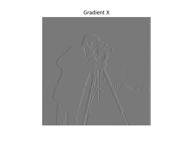
Gradient X (Cameraman)

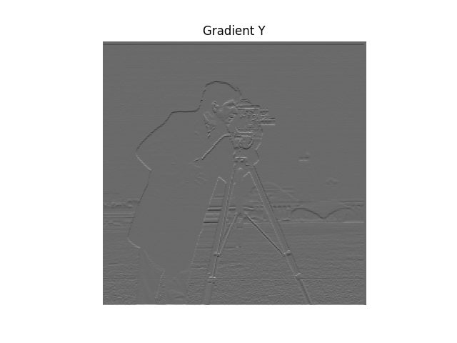
Gradient Y (Cameraman)

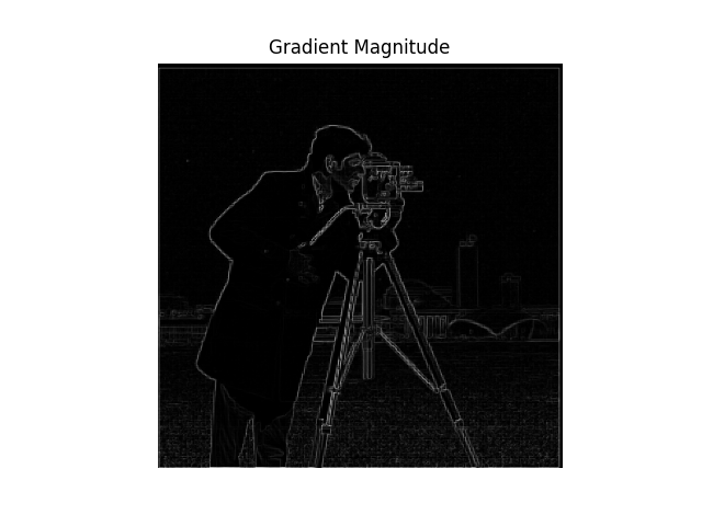
Gradient Magnitude (Cameraman)

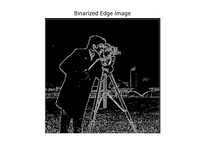
Binarized Edge Image (Cameraman)

1.2 Derivative of Gaussian (DoG) Filter

The finite difference approach produced noisy results, so to reduce noise and improve edge detection, a Gaussian blur can be applied to the image before calculating the gradients.

First, the image was smoothed using a Gaussian filter before applying the finite difference operators: \[ I_{\text{blurred}} = I * G \\ \frac{\partial I}{\partial x} = I_{\text{blurred}} * D_x \\ \frac{\partial I}{\partial y} = I_{\text{blurred}} * D_y \\ \nabla I = \sqrt{\left( \frac{\partial I}{\partial x} \right)^2 + \left( \frac{\partial I}{\partial y} \right)^2} \]

The Gaussian filter reduced noise and smoothed the image, leading to more refined edge detection. Additionally, by combining the Gaussian filter and derivative operators, I used Derivative of Gaussian (DoG) filters: \[ \text{DoG}_x = G * D_x, \quad \text{DoG}_y = G * D_y \] The DoG filters allowed for a more efficient and streamlined computation of edges, producing smoother results.

The DoG method improved the clarity of edges, especially in regions with noise or minor intensity variations. The smoothing effect from the Gaussian filter helped to reduce noise while still highlighting key structural details in the image.

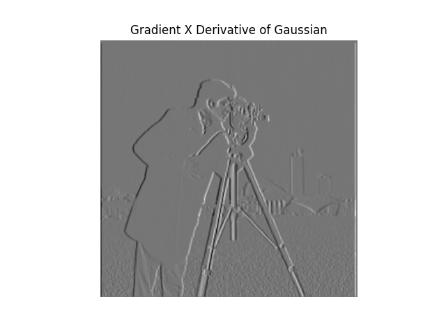
Gradient X (DoG) (Cameraman)

Gradient Y (DoG) (Cameraman)

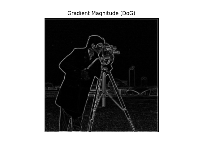
Gradient Magnitude (DoG) (Cameraman)

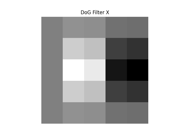
DoG Filter \( D_x \)

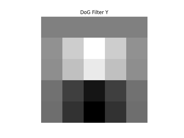
DoG Filter \( D_y \)

Part 2: Fun with Frequencies

2.1 Image Sharpening (Unsharp Masking)

Image sharpening enhances the edges and finer details in an image by increasing the presence of high-frequency components.

Using the unsharp masking technique, I first applied a Gaussian blur to the image, then subtracted the blurred version from the original to obtain the high-frequency details. The sharpening process is defined by: \[ I_{\text{sharpened}} = I + \alpha (I - I_{\text{blurred}}) \] The parameter \( \alpha \) controls the intensity of the sharpening effect.

When applied to slightly blurred images, this technique restored lost details effectively. However, when applied to already sharp images, over-sharpening resulted in noise amplification, making the image appear unnatural.

Unsharp masking worked well in recovering details in blurry images. However, careful tuning of the sharpening factor \( \alpha \) is required to avoid over-sharpening, which can lead to unwanted noise.

Original Image (Apple)

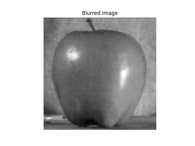
Blurred Image (Apple)

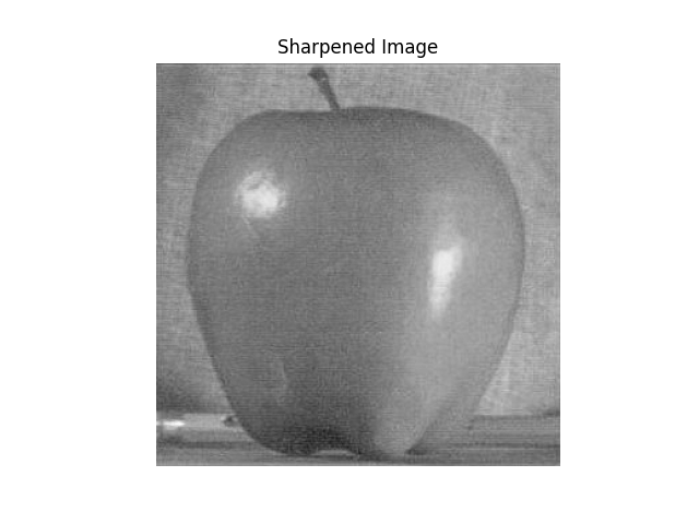
Sharpened Image (Apple)

Original Image (Owl)

Blurred Image (Owl)

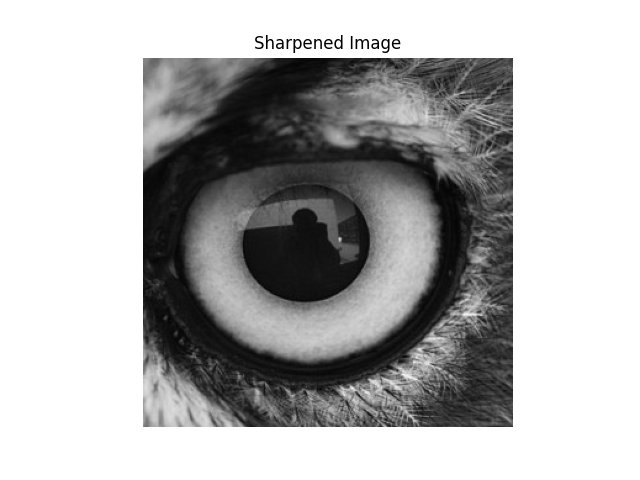
Sharpened Image (Owl)

2.2 Hybrid Images

Hybrid images combine the low-frequency components of one image with the high-frequency components of another. This technique creates a shift depending on the viewer's relative distance to the image: the high-frequency details dominate up close, while the low-frequency components become more obvious from further away.

The following steps were used to create a hybrid image: \[ I_{\text{low}} = I_1 * G, \quad I_{\text{high}} = I_2 - (I_2 * G) \] \[ I_{\text{hybrid}} = I_{\text{low}} + I_{\text{high}} \]

• Apple and Orange: \( \sigma_{\text{low}} = 2 \), \( \sigma_{\text{high}} = 4 \). The low-frequency components of the apple were extracted with moderate smoothing, while the high-frequency components of the orange were isolated using a stronger blur.
• Owl and Ball: \( \sigma_{\text{low}} = 3.5 \), \( \sigma_{\text{high}} = 10 \). The custom owl image required a higher sigma to smooth its intricate details, while the ball image was blurred significantly to capture only the high-frequency details for the hybrid.

The hybrid images demonstrated a visual phenomenon where different images appeared based on the viewing distance. However, the two images being properly aligned was critical to the success of the hybrid image.

While the hybrid technique produced good results, misalignment or incompatible features between the two images resulted in failure cases. Without a proper alignment of the images,it was difficult to achieve a smooth transition between the two frequency bands.

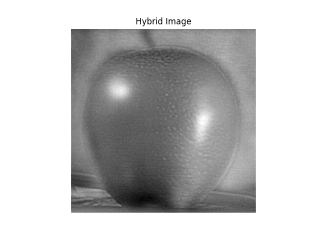
Hybrid Image (Apple and Orange)

2.3 Gaussian and Laplacian Stacks

Gaussian and Laplacian stacks are key tools in multiresolution image analysis, allowing for smooth blending of images at different scales.

A Gaussian stack is created by repeatedly applying Gaussian filters to the image, resulting in progressively blurred versions: \[ \text{Gaussian Stack} = \{ G_0, G_1, G_2, \dots, G_n \} \] The Laplacian stack isolates the high-frequency components between consecutive levels of the Gaussian stack: \[ \text{Laplacian Stack} = \{ L_0, L_1, L_2, \dots, L_{n-1} \}, \quad L_i = G_i - G_{i+1} \]

By using these stacks, I could blend images at different resolution levels, ensuring smooth transitions between the images without visible artifacts.

The Gaussian and Laplacian stacks were especially effective for image blending tasks, as they allowed for multiresolution analysis. This method enabled me to create seamless blends between different images across various frequency bands.

Gaussian Stack (Apple)

Laplacian Stack (Orange)

2.4 Multiresolution Blending

Multiresolution blending involves combining two images by blending their details at different scales. This technique uses Gaussian and Laplacian stacks to gradually blend images, resulting in a smooth transition between the two. By using a mask that transitions from one image to the other, we can control which parts of each image dominate in the final output.

The blending process consists of the following steps:

• Create Gaussian stacks for the mask to control the blending at multiple scales.
• Create Laplacian stacks for both images to capture their details at different frequency levels.
• Blend the corresponding Laplacian levels of both images using the Gaussian mask at each level.
• Reconstruct the final blended image by combining the blended Laplacian stack levels.

For this experiment, I used a simple horizontal mask where the left half of the mask was filled with 1s and the right half with 0s. This resulted in a smooth left-to-right transition between the two images that attempts to replicate the findings of the "spline83" paper.

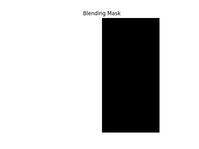
Blending Mask

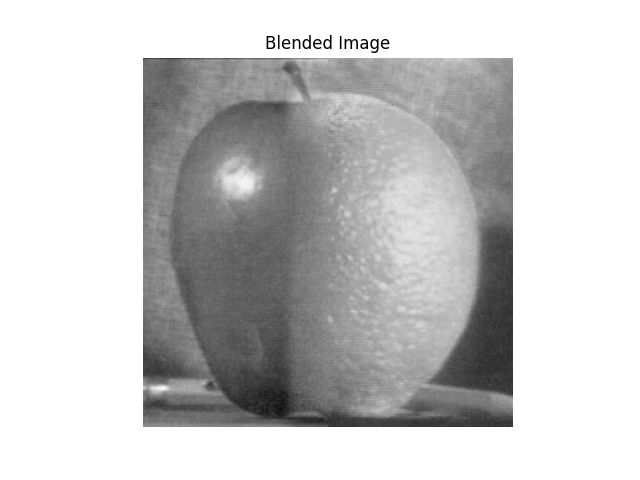
Blended Image (Apple and Orange)

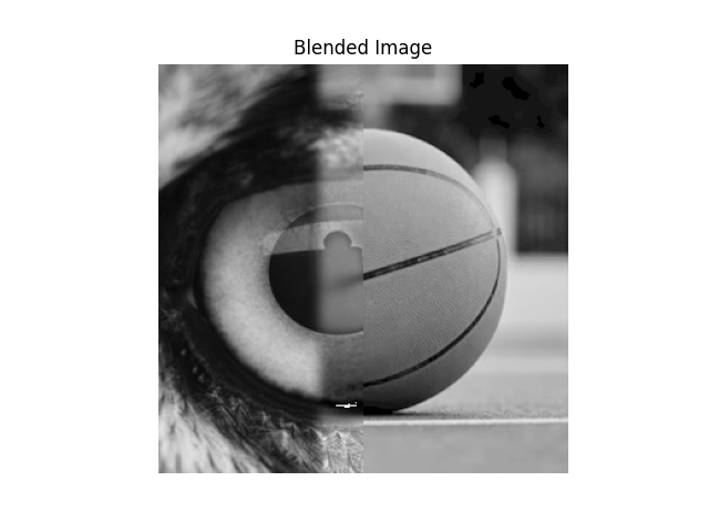
[Failure] Blended Image (Owl Eye and Basketball)

The multiresolution blending technique enabled smooth, seamless transitions between two images by using a Gaussian mask to blend details at multiple scales, preventing abrupt changes or visible seams. This method is particularly effective for combining images with varying textures, lighting conditions, or focus areas. Additionally, fine-tuning the mask allows for creative control over the blend's smoothness and areas of influence.

To address the failure case with my custom images, not every mask seemed to be compatible with my current Laplacian and Gaussian stacking, as the process is highly dependent on the images being used. Without proper fine-tuning of the mask and variables involved, the blend's smoothness can sometimes appear relatively rough.

Conclusion

This project gave me the chance to dive into various image processing techniques, from edge detection with finite difference and DoG filters to blending images using Gaussian and Laplacian stacks. Since I regularly use programs like Adobe Photoshop and Lightroom, it was really interesting to see the math and algorithms behind the tools I use every day. Understanding how different frequencies affect image clarity, detail, and blending helped me appreciate the concepts that make these software applications function.